Quick Answer
At GCR 0.64, annual beam shading loss in landscape orientation at 20° tilt runs at 1.5%. Over 25 years at a conservative 2% annual electricity price escalation, that gap is approximately $26,000 in present-value lost revenue on a 100 kWp system. A 100 kWp ground-mount at GCR 0.40 requires roughly 20% more land than the same system at GCR 0.50.
Spacing errors are the silent underperformer on solar projects. A row pitch that is 0.3 m too narrow on a 200 kWp commercial ground-mount can reduce annual yield by 4–6 percentage points — losses that compound every year for 25 years. At $0.10/kWh, that is thousands of dollars in lost revenue that no module upgrade, no inverter optimization, and no O&M program can recover. The calculation itself takes five minutes once you know the formula. The problem is that most spreadsheet-based workflows get at least one input wrong. Also see: Us Residential Solar Market Trends 2026. For United States-specific compliance details, see United States arizona/phoenix.
At GCR 0.64, annual beam shading loss in landscape orientation at 20° tilt runs at 1.5%. Over 25 years at a conservative 2% annual electricity price escalation, that gap is approximately $26,000 in present-value lost revenue on a 100 kWp system. A 100 kWp ground-mount at GCR 0.40 requires roughly 20% more land than the same system at GCR 0.50.
Good solar software automates this calculation in real time, connecting tilt angle, module geometry, and latitude to a live spacing result as you design. But even if your solar design software handles spacing automatically, understanding the underlying math is what separates a competent designer from one who can defend every number on a client’s proposal.
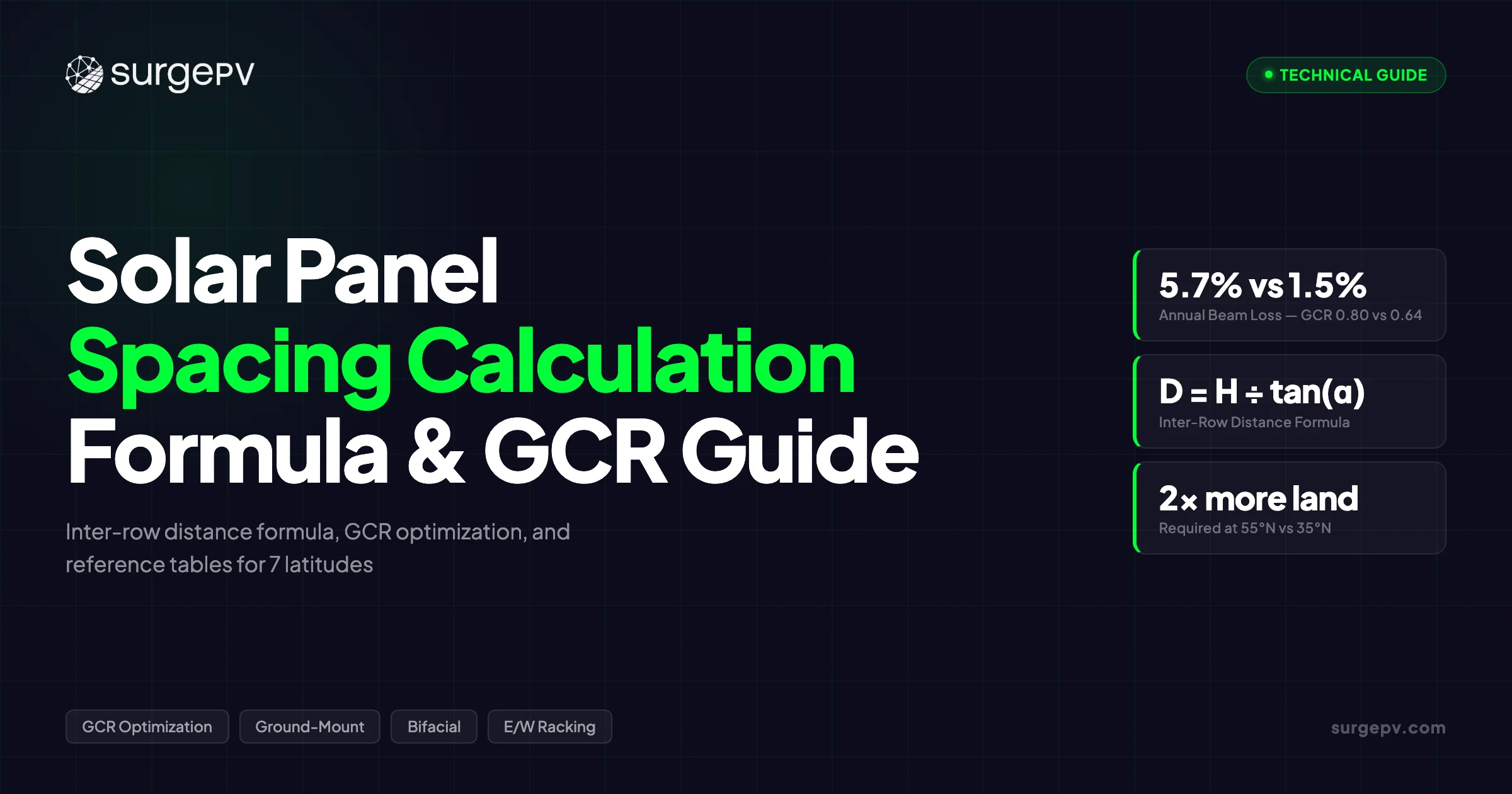
This guide covers the full solar panel spacing calculation from first principles: the inter-row distance formula, Ground Cover Ratio optimization using NREL published data, quick-reference tables for 7 latitudes, and specific guidance for ground-mounted, flat-roof, bifacial, and east-west racking configurations. Read Bifacial Solar Panel Design Guide for a complete walkthrough.
TL;DR — Solar Panel Spacing Calculation
At GCR 0.80 versus 0.64, inter-row beam shading loss shifts from 1.5% to 5.7% — the difference between a well-performing system and one that underperforms its financial model by thousands of dollars over 25 years. NREL data (TP-6A20-62471) shows that at GCR 0.80 vs. 0.64, annual beam loss nearly quadruples in landscape orientation at 20° tilt.
In this guide:
- Why spacing errors cost real money — revenue impact table with real kWh numbers
- The complete solar panel spacing formula, step by step with worked examples
- Ground Cover Ratio explained with NREL shading loss data by GCR value
- Spacing requirements by installation type: ground-mount, flat roof, residential pitched roof
- Portrait vs. landscape orientation — impact on H, D, and row pitch
- Bifacial module spacing requirements and albedo values by surface type
- East-west racking — when the formula changes completely
- Ten common spacing mistakes with exact consequences
- How solar design software handles spacing automatically
Why Spacing Calculation Errors Cost Real Money
The financial case for getting spacing right starts with the NREL shading loss data. At GCR 0.64, annual beam shading loss in landscape orientation at 20° tilt runs at 1.5%. At GCR 0.80, it rises to 5.7%. That 4.2 percentage-point difference is not a rounding error — it is a compounding revenue gap.
| Scenario | GCR | Annual Beam Loss | Lost kWh (100 kWp, 5.5 peak-sun-hrs) | Revenue Lost at $0.10/kWh |
|---|---|---|---|---|
| Optimal spacing | 0.64 | 1.5% | ~3,011 kWh | ~$301/year |
| Dense spacing | 0.80 | 5.7% | ~11,443 kWh | ~$1,144/year |
Basis: 100 kWp × 5.5 peak-sun-hours × 365 days = 200,750 kWh/yr baseline.
The difference between those two scenarios — $843/year — does not sound dramatic on a single-year budget. Over 25 years at a conservative 2% annual electricity price escalation, that gap is approximately $26,000 in present-value lost revenue on a 100 kWp system. Scale to a 500 kWp project and the number exceeds $130,000.
Over-spacing carries its own cost. On ground-mounted systems, wasted land area directly increases lease expense. Typical commercial land lease rates run $500–$2,000 per acre per year depending on location and lease structure (SmartEnergyUSA, 2026; AgWeb, 2024). A 100 kWp ground-mount at GCR 0.40 requires roughly 20% more land than the same system at GCR 0.50. At $1,000/acre/year, that is $500–$1,500 in unnecessary annual lease cost for a small commercial system — a number that also compounds.
For more details, see our guide on solar panel recycling in Europe. Also see: European Solar Incentives. For Europe-specific compliance details, see Europe solar compliance.
The ten most common spacing mistakes, covered in detail later in this guide, share a common thread: they all reduce to either using the wrong input value in the formula, or applying a formula designed for one installation type to a different one. The formula itself is not complex. Here is how it works.
The Solar Panel Spacing Formula, Step by Step
The inter-row spacing calculation has three steps. Each step feeds directly into the next. Do them in order.
Step 1 — Calculate Effective Panel Height (H)
Effective panel height (H) is the vertical height of the shadow cast by one row of panels. It is not the physical panel height — it is the panel’s dimension in the tilt direction multiplied by the sine of the tilt angle.
H = L × sin(β)

Where:
  L = module dimension in the tilt direction
      (length for portrait orientation, width for landscape)
  β = tilt angle in degrees from horizontal
Worked example 1 — Portrait orientation: 72-cell module, L = 2,000 mm (the long dimension, facing up the tilt), β = 20°.
H = 2,000 × sin(20°)
H = 2,000 × 0.342
H = 684 mm = 0.684 m
Worked example 2 — Landscape orientation: Same 72-cell module, now rotated 90°. L = 1,000 mm (the short dimension now faces up the tilt), β = 20°.
H = 1,000 × sin(20°)
H = 1,000 × 0.342
H = 342 mm = 0.342 m
Landscape orientation cuts effective shading height exactly in half at any given tilt angle. This is why landscape layouts allow tighter row pitch on dense commercial rooftops — the shadow cast is shorter, so less horizontal clearance is needed before the next row begins. On a 10,000 m² urban rooftop where every meter of row pitch translates to 2–3 fewer rows of panels, that 50% reduction in H is a significant capacity gain.
Step 2 — Find the Winter Solstice Solar Elevation Angle (α)
The design standard is shade-free performance at winter solstice solar noon. December 21st has the lowest solar elevation angle of the year. If each row clears its neighbor’s shadow on that day at solar noon, it stays clear for every other day of the year.
α = 90° − Latitude − 23.45°

(solar elevation at winter solstice solar noon, true south azimuth)
The 23.45° term is the Earth’s axial tilt — the sun’s maximum declination from the equator.
| Latitude | City Reference | α (Winter Solstice Noon) |
|---|---|---|
| 35°N | Los Angeles / Seville | 31.6° |
| 40°N | Denver / Madrid / Naples | 26.6° |
| 42°N | Boston | 24.6° |
| 45°N | Minneapolis / Milan / Lyon | 21.6° |
| 50°N | London / Prague | 16.6° |
| 52°N | Berlin / Amsterdam | 14.6° |
| 55°N | Copenhagen | 11.6° |
Note on the design window: Solar noon α is the maximum sun angle on December 21st. For commercial and C&I projects, the design standard is typically a shade-free window from 9 AM to 3 PM, not just solar noon. The 9 AM winter solstice elevation angle is 5–15° lower than the noon value depending on latitude. This produces a more conservative (larger) D — typically 20–35% wider spacing than a solar-noon-only calculation. For Boston (42°N), the 9 AM–3 PM design window angle drops from 24.6° to approximately 19.5°. Always use the design-window angle for C&I projects unless the client accepts a shorter daily shade-free window.
Step 3 — Calculate Minimum Row Spacing and Row Pitch
With H and α known, the minimum inter-row spacing and full row pitch follow directly.
D = H ÷ tan(α)        [minimum row spacing, trailing edge to leading edge]
P = D + (W × cos(β))  [full row pitch, trailing edge to trailing edge]
GCR = W ÷ P           [Ground Cover Ratio]

Where:
  D = minimum inter-row spacing (m)
  H = effective panel height from Step 1 (m)
  α = solar elevation angle from Step 2 (°)
  P = row pitch (m)
  W = module width (horizontal dimension when installed)
  β = tilt angle (°)
Azimuth correction: If rows are not oriented true south, apply: D_corrected = D × cos(azimuth_deviation). A 10° off-south azimuth changes D by approximately 1.5% — negligible on residential systems. On a large ground-mount where land lease costs are calculated per acre, a 20° off-south azimuth deviation changes D by about 6%, which is worth tracking in the layout model.
Worked Example — 72-Cell Module at 35°N, 20° Tilt
Scenario: 100 kWp ground-mounted system, Los Angeles (35°N), 20° tilt, south-facing, 72-cell modules (2,000 × 1,000 mm), portrait orientation, solar noon design window.
GIVEN:
  Module: 72-cell — 2,000 mm (L, portrait) × 1,000 mm (W)
  Tilt (β): 20°
  Latitude: 35°N
  Orientation: Portrait, true south

STEP 1: Effective height
  H = 2,000 × sin(20°) = 2,000 × 0.342 = 684 mm = 0.684 m

STEP 2: Winter solstice solar elevation
  α = 90° − 35° − 23.45° = 31.55° ≈ 31.6°

STEP 3: Minimum row spacing
  D = 0.684 ÷ tan(31.6°) = 0.684 ÷ 0.615 = 1.11 m

STEP 4: Full row pitch
  P = D + (W × cos(β)) = 1.11 + (1.000 × cos(20°)) = 1.11 + 0.940 = 2.05 m

STEP 5: Ground Cover Ratio
  GCR = W ÷ P = 1.000 ÷ 2.05 = 0.49

RESULT: 2.05 m row pitch, GCR 0.49 — within the low-shading zone.
Now run the same module and tilt across four latitudes to see how D and GCR shift with location:
| Latitude | City | α | D (m) | Row Pitch (m) | GCR |
|---|---|---|---|---|---|
| 35°N | Los Angeles | 31.6° | 1.11 | 2.05 | 0.49 |
| 40°N | Denver | 26.6° | 1.38 | 2.32 | 0.43 |
| 45°N | Minneapolis | 21.6° | 1.74 | 2.68 | 0.37 |
| 50°N | London | 16.6° | 2.32 | 3.26 | 0.31 |
Pro Tip
At 50°N, minimum row spacing more than doubles compared to 35°N. A 1 MW project in London needs roughly 60% more land than an equivalent system in Los Angeles to achieve the same shading threshold. This is not a design preference — it is the geometry of the sun angle at that latitude.
Row pitch is the output of the spacing formula, but it is not the final decision variable. GCR is the variable that ties spacing directly to business outcomes — land cost, capacity density, shading losses, and financial returns. That is where the real optimization work happens.
Ground Cover Ratio (GCR) — The Variable That Ties Spacing to Yield
GCR is where spacing decisions become financial decisions. Getting the formula right is necessary but not sufficient; optimizing GCR for your site, latitude, and installation type is what separates a competitive proposal from one that leaves yield or land efficiency on the table.
What Is GCR and Why It Matters
GCR = Module Width ÷ Row Pitch
Range: 0.25 (sparse) to 0.85 (dense)
GCR is the fraction of the ground area covered by panels. GCR 0.5 means panels cover half the available ground. GCR 0.8 means 80% of the ground is covered. The GCR trade-off is direct: higher GCR produces more capacity per acre and lower land cost per kW installed, but generates higher inter-row shading losses. Lower GCR reduces shading and preserves yield, but increases land requirement and lease cost per kW.
Neither extreme is right. The optimal GCR depends on the site’s latitude, electricity price, and land lease rate — and it can be calculated, not guessed.
NREL Shading Loss by GCR
NREL Technical Report TP-6A20-62471 provides measured beam shading loss by GCR for a south-facing fixed-tilt array at 20° tilt in Sacramento (approximately 38°N). The table below extends the NREL data with a revenue-impact calculation based on a 100 kWp system at 5.5 peak-sun-hours.
| GCR | Row Spacing | Annual Beam Loss — Landscape | Annual Beam Loss — Portrait | Lost kWh per 100 kWp | Revenue Lost at $0.10/kWh |
|---|---|---|---|---|---|
| 0.64 | 4.6 m | 1.5% | 2.3% | ~3,011 kWh | ~$301/yr |
| 0.74 | 4.0 m | 3.7% | 5.6% | ~7,428 kWh | ~$743/yr |
| 0.80 | 3.7 m | 5.7% | 8.6% | ~11,443 kWh | ~$1,144/yr |
Basis: 100 kWp × 5.5 peak-sun-hours × 365 days = 200,750 kWh/yr. Landscape loss column used for kWh and revenue calculation.
Moving from GCR 0.64 to GCR 0.80 increases annual beam loss by 4.2 percentage points in landscape. On a 500 kWp system, that is approximately 42,000 kWh per year — about $4,200/year at $0.10/kWh, every year for 25 years. In present value terms at a 6% discount rate, that is roughly $54,000 in lost revenue from a spacing decision made in the design stage.
Note on Latitude Adjustment
The NREL data is calibrated for Sacramento (latitude ~38°N). At higher latitudes, the same GCR values produce proportionally higher shading losses because the sun angle is lower. The GCR sweet spot shifts toward 0.30–0.45 as you move north of 45°N. Do not apply Sacramento GCR benchmarks directly to Berlin or Copenhagen sites.
For the latest details on Germany, see Community Solar Projects Germany.
Optimal GCR Ranges by System Type
| System Type | Typical GCR Range | Notes |
|---|---|---|
| Ground-mounted fixed tilt, 45–55°N | 0.30–0.45 | Winter sun angle constrains spacing |
| Ground-mounted fixed tilt, 35–44°N | 0.40–0.55 | Sacramento-style conditions |
| Commercial flat roof (portrait) | 0.40–0.55 | 2.14–2.45 m pitch |
| Commercial flat roof (landscape) | 0.55–0.70 | 1.26–1.75 m pitch |
| Bifacial ground-mounted | 0.30–0.50 | Wider spacing preserves rear-side irradiance |
| Single-axis tracker | 0.25–0.40 | Wider needed for rotation sweep |
These ranges are starting points. Final GCR should be confirmed by running sensitivity analysis on your specific combination of latitude, electricity price, and land cost. The financial breakeven between land savings and shading losses shifts by latitude — at 52°N, the shading-loss penalty for increasing GCR from 0.40 to 0.50 is significantly steeper than it is at 38°N.
Spacing by Installation Type
Ground-Mounted Fixed Tilt Systems
Ground-mounts offer the most design flexibility and the most consequences for spacing errors. Typical row pitch ranges from 3–6 m depending on latitude and tilt angle — but pitch is not the only driver.
Maintenance access requires a minimum of 0.5–1.0 m clear between row trailing edge and next row’s leading edge beyond the shading-minimum D. Cleaning vehicles and mowing equipment typically need 3.0 m clear lanes every 3–4 rows on larger arrays. On a 1 MW+ system, these operational clearance requirements often govern final row pitch more than the shading calculation — particularly in regions where vegetation management is part of the O&M scope.
Practical starting point: For ground-mounts above 40°N, begin at GCR 0.40 and test financial sensitivity across GCR 0.35–0.50 before locking in pitch. Below GCR 0.35, land lease costs typically outpace the shading-loss savings at most US and European electricity prices. Above GCR 0.55 at these latitudes, shading losses start compounding materially.
IEC 62548 covers PV array design and installation spacing; NEC Article 690 governs electrical safety for US PV systems. Neither standard mandates specific inter-row distances, though project documentation typically includes a shading analysis. A spacing calculation backed by the D = H ÷ tan(α) formula and the NREL GCR data is sufficient documentation on most AHJ submittals.
Commercial Flat Rooftop Systems
Flat-roof commercial systems flip the optimization. The roof area is fixed, so the goal is the highest GCR that keeps shading losses within the project’s financial model tolerance. Over-spacing on a flat roof means fewer panels and lower capacity — the opposite problem from a ground-mount.
Typical row pitch numbers from commercial racking suppliers: portrait orientation, 2.14–2.45 m pitch at 10–15° tilt. Landscape orientation, 1.26–1.75 m pitch at equivalent tilt (KB Racking, 2025).
Tilt angle is a key lever on flat roofs. Lowering tilt from 20° to 10° reduces H by roughly 40%, which cuts required D proportionally and fits more capacity per m². The per-panel yield cost of 10° vs. 20° tilt is approximately 3–5% in most mid-latitude locations. For a dense urban rooftop, fitting 15% more capacity at 4% less per-panel yield is almost always the better financial outcome.
Worked comparison — 10° vs. 20° tilt on a 1,000 m² roof: At 10° tilt, portrait row pitch drops from 2.45 m to approximately 1.85 m. That reduction in pitch allows approximately 15% more panel rows on the same roof area. Even with a 4% per-panel yield penalty from suboptimal tilt, total annual generation increases by roughly 10–11%. On a 200 kWp baseline, that is an additional 20 kWp capacity and 20,000–22,000 kWh/year — worth approximately $2,000–$2,200/year at $0.10/kWh. For France-specific information, see Agricultural Solar Case Study. For the latest details on France, see Floating Solar Farms France.
Pro Tip
Many C&I designers set flat-roof tilt at 10–15° rather than the latitude-optimal 30–35°. The reduced shadow saves more capacity than the suboptimal tilt costs in most dense urban rooftop scenarios. Run both cases in your simulation before finalizing the proposal.
Residential Pitched Rooftop Systems
On a standard pitched roof, inter-row shading between strings is rare. The main spacing concerns are edge setbacks, eave gaps, and fire code setbacks — typically 0.5–1.5 m from ridge lines, valleys, and roof edges depending on jurisdiction. Local fire codes govern these setbacks.
Inter-row spacing becomes relevant on residential projects in one specific scenario: portrait stacking on long roof faces — common on large custom homes, warehouses converted to residential, or solar carport structures. When stacking portrait rows on a long pitched roof, use the sun elevation angle at the first or last generation hour (rather than solar noon) as α. This produces more conservative spacing that ensures useful morning and afternoon generation, not just a midday shade-free window. See Commercial Solar Carport Design Guide for detailed guidance.
Portrait vs. Landscape — Impact on Spacing and GCR
Orientation choice directly changes H, D, and the entire row pitch calculation. On commercial systems it is an engineering variable with measurable financial consequences — not a stylistic decision.
| Parameter | Portrait | Landscape |
|---|---|---|
| Effective height H (72-cell module, 20° tilt) | 684 mm | 342 mm |
| Minimum row spacing D at 35°N | 1.11 m | 0.56 m |
| NREL annual beam loss at GCR 0.74 | 5.6% | 3.7% |
| Typical row pitch — commercial flat roof | 2.14–2.45 m | 1.26–1.75 m |
Landscape halves effective shading height, cuts minimum row spacing by approximately 50%, and reduces NREL beam loss by roughly 1.9 percentage points at equivalent GCR. On a dense commercial flat rooftop where the roof area is the binding constraint, landscape consistently allows 20–40% more installed capacity than portrait at the same shading-loss tolerance.
When to choose landscape: Dense commercial flat rooftops where roof area is limited and capacity maximization is the priority. Urban warehouses, logistics centers, supermarkets. Landscape is the standard choice when GCR needs to exceed 0.55.
When to choose portrait: Ground-mounts and large-footprint roofs where GCR is already low (0.40–0.50) and longer portrait strings reduce combiner count and DC wiring cost. Portrait is also standard for residential pitched roofs.
Key Finding — NREL Portrait vs. Landscape
NREL data shows portrait configuration has 50–65% higher beam shading loss than landscape at the same GCR. On a dense urban rooftop where capacity is the priority, landscape is often the better engineering choice — not just a layout preference.
Bifacial Solar Panel Spacing Requirements
Why Bifacial Modules Need Different Spacing
Bifacial modules generate energy from both front and rear surfaces. The rear gain depends on reflected irradiance from the ground — and that reflected irradiance drops sharply if the module is too close to the ground, the GCR is too high, or the ground surface has low albedo.
These three factors interact. A bifacial array with optimal front-side spacing but high GCR still loses rear gain because the panels shade their own ground footprint, reducing the reflected light available to the rear surface. The result: bifacial systems require wider spacing than equivalent monofacial systems to capture the full bifacial yield benefit.
Preferred GCR for bifacial: 0.30–0.50, wider than equivalent monofacial designs. IEEE and NREL research (NREL, 2016; IEEE Journal of Photovoltaics, 2015) cites approximately 1.0–1.5 m ground clearance from module bottom edge as the range where rear-side irradiance is near optimal. Below 0.6 m clearance, rear gain drops significantly depending on GCR and albedo.
The shade-free spacing check uses the same formula: D = H ÷ tan(α). Apply that first, then run a rear-irradiance check using the system’s bifacial simulation model to confirm the clearance and GCR combination delivers the expected rear gain. For most bifacial ground-mounts, the rear-irradiance clearance check produces wider spacing than the shading formula alone.
Albedo Values by Surface Type
Ground surface albedo directly determines how much reflected light reaches the module’s rear. The difference between a dark soil site (albedo 0.05) and a white gravel site (albedo 0.60) can be 4–8% in absolute annual energy yield on a bifacial system.
| Ground Surface | Albedo Value |
|---|---|
| Fresh snow | 0.80–0.90 |
| White concrete / membrane | 0.60–0.80 |
| Light gravel | 0.50–0.70 |
| Grass (dry) | 0.20–0.30 |
| Asphalt | 0.10–0.20 |
| Dark soil | 0.05–0.15 |
Ground treatment is an EPC scope decision, not just a simulation input. Specifying light crushed limestone or white gravel under a bifacial array costs $2–$5/m² as a one-time materials cost (HomeGuide, 2025). At $0.10/kWh and 1 MWp, a 3–6% annual yield improvement is worth $3,000–$6,000/year — a payback of one to two years on the ground treatment cost.
Pro Tip
For C&I ground-mounts with bifacial modules, specify the ground treatment material in the EPC scope document. Leaving it as “bare soil” when the final site will have gravel permanently reduces rear-side yield — and it cannot be corrected after commissioning without a costly retrofit.
East-West Racking Spacing — When the Formula Changes Completely
How E/W Geometry Differs From South-Facing Arrays
In a south-facing array, every row casts a shadow that falls on the row immediately behind it. This is what the D = H ÷ tan(α) formula is designed to prevent. In east-west racking, panels face east and west from a central ridge. The shadow from an east-facing panel falls away from the west-facing panel — in the opposite direction. The two panel faces never shade each other.
The result: inter-row gap between east-facing and west-facing module backs is 0.01–0.40 m, versus 2–6 m for south-facing ground-mounts at equivalent latitudes. The standard south-facing spacing formula does not apply to E/W racking. Applying it produces massive over-spacing that defeats the entire purpose of the E/W layout.
Capacity advantage: E/W racking increases flat-roof capacity by 20–30% versus south-facing portrait at the same GCR target. On a 1,000 m² rooftop where south-facing portrait fits 80 kWp, E/W typically fits 100–110 kWp.
Yield trade-off: Each panel tilts 10–15° toward east or west rather than optimal south. Per-panel output is approximately 3–7% lower than a south-facing system at the same tilt angle. For most commercial flat rooftops where energy target is the primary KPI, the capacity gain from fitting more panels dominates the per-panel yield loss.
| Parameter | South-Facing Portrait 20° | E/W Racking 12° |
|---|---|---|
| Row pitch | 2.30 m | 0.35 m |
| Panels fitted | ~200 × 400W = 80 kWp | ~260 × 400W = 104 kWp |
| Per-panel yield vs. optimal south | Baseline | ~5% lower |
| Estimated net capacity | 80 kWp | 104 kWp (+30%) |
| Estimated annual generation | 100 MWh | 124 MWh |
Based on 1,000 m² flat roof, 400W modules, 2,000 × 1,000 mm.
When to recommend E/W: Dense urban commercial rooftops with high capacity targets and limited south-facing area. E/W is the standard choice for logistics centers, factories, and supermarkets with large flat roofs. It is not appropriate for ground-mounts, residential pitched roofs, or sites with significant south-facing tilt already built into the structure.
E/W Spacing Clarification
The 0.01–0.40 m inter-row gap for E/W racking looks incorrect to engineers trained on south-facing arrays. The geometry is correct — east and west panels tilted at 10–15° do not shade each other when oriented back-to-back. The near-zero gap is not an error in the racking specification.
Ten Common Solar Panel Spacing Mistakes
These are the systematic errors that appear across manual spreadsheet-based workflows. Each one has a specific, measurable consequence.
-
Using solar noon α instead of the 9 AM–3 PM design window. Solar noon gives the highest (most favorable) sun angle on December 21st, which produces the shortest D. Commercial and C&I projects typically require a shade-free window from 9 AM to 3 PM. The 9 AM winter solstice angle is lower than noon by 5–15° depending on latitude — this increases required D by 20–35%. A design calculated at solar noon and built to that pitch will have shaded panels for 2–4 hours on winter mornings and afternoons.
-
Ignoring portrait vs. landscape in the H calculation. A 72-cell module in portrait has twice the effective shading height as the same module in landscape at identical tilt. Calculating H for landscape orientation and using that value to set portrait row pitch produces spacing roughly 50% too tight — which translates directly to 3–5% additional annual beam shading loss at equivalent GCR.
-
Using module width instead of module length in the tilt direction. For portrait orientation, L in H = L × sin(β) is the module’s longer dimension, not the shorter one. Reversing the two dimensions is the single most common manual calculation error on residential and small commercial projects. The result is an H value roughly half the correct value, and a D that is dangerously tight.
-
Applying a mid-latitude GCR reference to a high-latitude site. NREL’s GCR loss data is calibrated for Sacramento (~38°N). At Berlin (52°N) or Copenhagen (55°N), the same GCR produces dramatically higher shading losses because the winter sun angle is much lower. A GCR of 0.55 that works acceptably in Los Angeles generates 2–3× higher beam shading loss in northern Europe. Never apply a GCR benchmark from a different climate zone without recalculating D for the actual site latitude.
-
Forgetting maintenance clearance on ground-mounted systems. The formula gives the shading-minimum D — the absolute minimum for shade-free operation. Real installations need at least 0.5–1.0 m added for a maintenance worker to access, inspect, and clean panels without stepping on adjacent rows. Large-scale commercial sites often need 3.0 m clear lanes every 3–4 rows for cleaning vehicles. Omitting maintenance clearance produces a layout that is technically shade-free and practically unserviceable.
-
Not specifying ground surface in bifacial projects. Rear-side yield on a bifacial module varies by 6–10% absolute depending on albedo. Specifying “bare soil” in the simulation when the final site will have gravel or concrete leaves 4–8% annual yield permanently on the table — and it cannot be corrected after commissioning without excavating and re-covering the ground under a live array.
-
Treating E/W racking like south-facing arrays. Applying south-facing spacing calculations to an E/W system produces massive over-spacing and loses the entire capacity advantage of E/W racking. The 0.01–0.40 m inter-row gap for E/W is not a mistake — it is the correct answer. Engineers new to E/W should verify against the racking manufacturer’s application guide before finalizing the layout.
-
Ignoring azimuth deviation from true south. A 20° off-south azimuth changes effective D by about 6%. On residential systems, this is below the threshold of practical concern. On a 5+ MW ground-mount, the cumulative error in land area sizing becomes significant enough to affect lease agreement boundaries. Large ground-mounts oriented off-south due to parcel geometry should apply the azimuth correction factor to D before calculating land area.
-
Using module dimensions from memory rather than the datasheet. 60-cell and 72-cell are reference categories, not fixed physical dimensions. A “72-cell” module from different manufacturers can range from 1,956 mm to 2,094 mm in the tilt direction (Oushang Solar, n.d.; LONGi Solar, n.d.). A 40 mm difference in L changes H by approximately 14 mm at 20° tilt — small per row, significant when compounded across a multi-row layout. Always pull the current datasheet before running spacing calculations, particularly when substituting modules mid-project.
-
Not rechecking spacing after a mid-project module substitution. Module swaps during procurement, common when supply chain delays force substitutions, change L, H, D, GCR, and all downstream spacing decisions. A module that is 40 mm longer in the tilt direction changes D by 2–3 cm at 20° tilt, which compounds across a multi-row layout into meaningful land area and row count changes. Any module substitution after the layout is set should trigger a full spacing recalculation before construction begins.
For more details, see our guide on solar supply chain trends.
All ten errors are systematic — they come from manual spreadsheet calculations applied without the full parameter set visible in one place. The solution is not more careful spreadsheet work. It is automating the calculation at the design stage, where every input is locked to the actual module datasheet and site coordinates.
How Solar Design Software Handles Spacing Automatically
What Automated Spacing Calculation Actually Does
Physics-based 3D irradiance simulation recalculates shading at every hour of the year — 8,760 hourly intervals, not just a single winter solstice snapshot. The solar shadow analysis software models actual module geometry, terrain elevation, and adjacent obstructions across the full annual sun path. GCR becomes a live output of the layout as modules are placed, not a pre-calculated input entered into a separate cell.
String sizing, bill of materials, and the financial model all connect to the same layout. When row pitch changes by 0.2 m, annual yield updates immediately. There is no translation step between the spacing calculation and the financial model — they are the same model.
The difference matters for proposals as much as for design. A manually calculated GCR entered into a financial spreadsheet is a static assumption. A simulation-driven GCR tied to actual module placement is a defensible output — one that updates automatically when the client asks “what if we add two more rows?”
How SurgePV’s Shadow Analysis Tool Handles This
SurgePV’s solar design software renders a physics-based 3D model of the site. Place modules on the model and inter-row shading calculates across the full annual sun path — not a simplified solstice check. The generation and financial tool connects directly to the layout: adjusting row pitch by 0.2 m immediately updates annual yield, payback period, and IRR without opening a separate spreadsheet. For a direct comparison, see Arka 360 vs SurgePV.
The platform handles residential and C&I projects in the same workspace. Clara AI assists with layout optimization, including inter-row spacing recommendations based on the site’s latitude, tilt angle, and module selection. No desktop install required — cloud-based, accessible from any device on site or in the office.
Stop Calculating Row Spacing in Spreadsheets
SurgePV’s shadow analysis tool models inter-row shading across the full annual sun path — not just winter solstice noon. Design, simulate, and propose in one tool.
Book a DemoNo commitment required · 20 minutes · Live project walkthrough
Solar Panel Spacing Quick-Reference Tables
Use these tables as a starting point for any new project. All values assume true south orientation and solar noon design window. Add 20–35% to D for a 9 AM–3 PM commercial design window.
Table 1 — Minimum row spacing by latitude 72-cell module, portrait orientation, 20° tilt, true south, solar noon design window:
| Latitude | City Reference | α | H (m) | D_min (m) | Full Row Pitch (m) | GCR |
|---|---|---|---|---|---|---|
| 35°N | Los Angeles | 31.6° | 0.684 | 1.11 | 2.05 | 0.49 |
| 40°N | Denver | 26.6° | 0.684 | 1.38 | 2.32 | 0.43 |
| 42°N | Boston | 24.6° | 0.684 | 1.49 | 2.43 | 0.41 |
| 45°N | Minneapolis | 21.6° | 0.684 | 1.74 | 2.68 | 0.37 |
| 50°N | London | 16.6° | 0.684 | 2.32 | 3.26 | 0.31 |
| 52°N | Berlin | 14.6° | 0.684 | 2.62 | 3.56 | 0.28 |
| 55°N | Copenhagen | 11.6° | 0.684 | 3.33 | 4.27 | 0.23 |
Table 2 — Typical spacing ranges by application:
| Installation Type | Typical Row Pitch | Typical GCR |
|---|---|---|
| Residential pitched roof | 0.5–1.5 m gap | N/A (roof geometry) |
| Commercial flat roof, portrait | 2.14–2.45 m | 0.40–0.55 |
| Commercial flat roof, landscape | 1.26–1.75 m | 0.55–0.70 |
| Ground-mounted fixed tilt, 35–40°N | 2.0–3.5 m | 0.40–0.55 |
| Ground-mounted fixed tilt, 45–55°N | 3.5–6.0 m | 0.25–0.40 |
| E/W racking (flat roof) | 0.10–0.40 m ridge-to-ridge | 0.65–0.80 |
| Bifacial ground-mounted | 3.0–5.0 m | 0.30–0.50 |
Table Usage Note
All values assume true south orientation (azimuth 180°) and a solar noon shade-free window. Adjust D upward by 20–35% for a 9 AM–3 PM commercial window, or downward for a narrower solar window if accepted by the client and AHJ.
Frequently Asked Questions
What is the standard spacing between solar panels?
There is no single standard spacing — it depends on latitude, tilt angle, and installation type. Ground-mounted systems in the US typically use 3–5 m row pitch depending on latitude and tilt. Commercial flat rooftops run 1.26–2.45 m depending on portrait vs. landscape orientation and the selected tilt angle. The correct spacing is calculated using D = H ÷ tan(α), where H is the module’s effective shading height and α is the solar elevation angle at winter solstice noon for the site’s latitude. Using a rule-of-thumb spacing without running this calculation for the actual site produces either over-spacing (wasted land) or under-spacing (shading losses).
How do I calculate inter-row distance for solar panels?
The calculation has two steps. First, calculate effective panel height: H = L × sin(β), where L is the module dimension in the tilt direction (long dimension for portrait, short dimension for landscape) and β is the tilt angle in degrees. Second, calculate minimum row spacing: D = H ÷ tan(α), where α is the winter solstice solar elevation angle at your latitude (α = 90° − latitude − 23.45°). Add the module’s horizontal footprint — module width × cos(tilt) — to D to get the full row pitch from trailing edge to trailing edge. For commercial projects, use the 9 AM–3 PM design window angle rather than solar noon, which increases D by 20–35%.
What is a good GCR for solar panels?
NREL data (TP-6A20-62471) shows GCR 0.64 produces only 1.5% annual beam shading loss in landscape orientation at 20° tilt. At GCR 0.80, that rises to 5.7% — nearly four times higher. For most commercial ground-mounts at 35–42°N, a GCR of 0.40–0.55 balances land efficiency against shading loss. Bifacial systems should target GCR 0.30–0.50 to preserve rear-side irradiance. Above 45°N, the shading-loss penalty for higher GCR values grows steeply — targets shift toward 0.30–0.45.
How far apart should solar panels be on a flat roof?
For portrait orientation on a commercial flat roof, typical row pitch is 2.14–2.45 m at 10–15° tilt. For landscape orientation, typical pitch is 1.26–1.75 m. Landscape spacing is roughly 40% tighter than portrait for equivalent shading performance — a meaningful capacity advantage on a fixed roof area. The exact value depends on your module dimensions, tilt angle, and local latitude. For E/W racking on a flat roof, the inter-row gap between east-facing and west-facing panel backs drops to 0.01–0.40 m — a completely different geometry from south-facing layouts.
Does solar panel tilt angle affect spacing?
Yes — directly, through the H calculation. A steeper tilt angle increases effective panel height (H = L × sin(β)), which increases the required minimum row spacing (D = H ÷ tan(α)). A 72-cell module at 30° tilt needs approximately 25% more row spacing than the same module at 20° tilt, at the same latitude. This is the core reason commercial flat-roof systems often use 10–15° tilt rather than the latitude-optimal 30–35°: lower tilt produces a shorter shadow, tighter row pitch, and more capacity per m² — a trade-off that favors lower tilt on most dense urban rooftops.
What is the solar panel spacing formula?
The standard formula set is: D = H ÷ tan(α), where D is the minimum row spacing, H = L × sin(β) is the module’s effective shading height (L = module dimension in tilt direction, β = tilt angle), and α is the solar elevation angle at winter solstice noon (α = 90° − latitude − 23.45°). Full row pitch P = D + (module width × cos(β)). GCR = module width ÷ row pitch. For the 9 AM–3 PM design window, replace α with the winter solstice sun elevation at 9 AM for your latitude — this is 5–15° lower than noon and produces 20–35% wider spacing.
Conclusion
Solar panel spacing calculation is a five-minute exercise with a 25-year financial tail. Getting it right at the design stage costs nothing. Getting it wrong costs yield every year of the system’s operating life — and no subsequent optimization can recover those losses.
Three action items to take from this guide:
- If you are sizing a ground-mounted system above 40°N, start with GCR 0.40 and use the NREL loss table to test sensitivity across GCR 0.35–0.50 before finalizing pitch. The shading-loss penalty for increasing GCR above 0.50 grows steeply north of 45°N — a Sacramento-calibrated benchmark does not transfer to northern European sites.
- For dense commercial flat rooftops, run both portrait and landscape orientations through the spacing calculation before fixing the layout. Landscape typically allows 20–40% more capacity at equivalent shading loss — a difference that changes the project’s financial case, not just its visual appearance.
- Check all ten common mistakes against your current design workflow. If you are still running spacing calculations in a spreadsheet, that is the error with the highest compounding cost — not because spreadsheets get the math wrong, but because they cannot update automatically when module dimensions, tilt angle, or site geometry change mid-project.
Design Your Next System With Spacing Built In
SurgePV calculates inter-row spacing, GCR, and annual shading loss in one physics-based simulation. No separate spreadsheet. Residential and C&I in the same tool.
Book a DemoNo commitment required · 20 minutes · Live project walkthrough
Once the spacing is right and the layout is confirmed, the next step is turning that design into a client-ready deliverable — solar proposal software connects directly to the design output so the proposal reflects the actual system, not a templated estimate.