Quick Answer
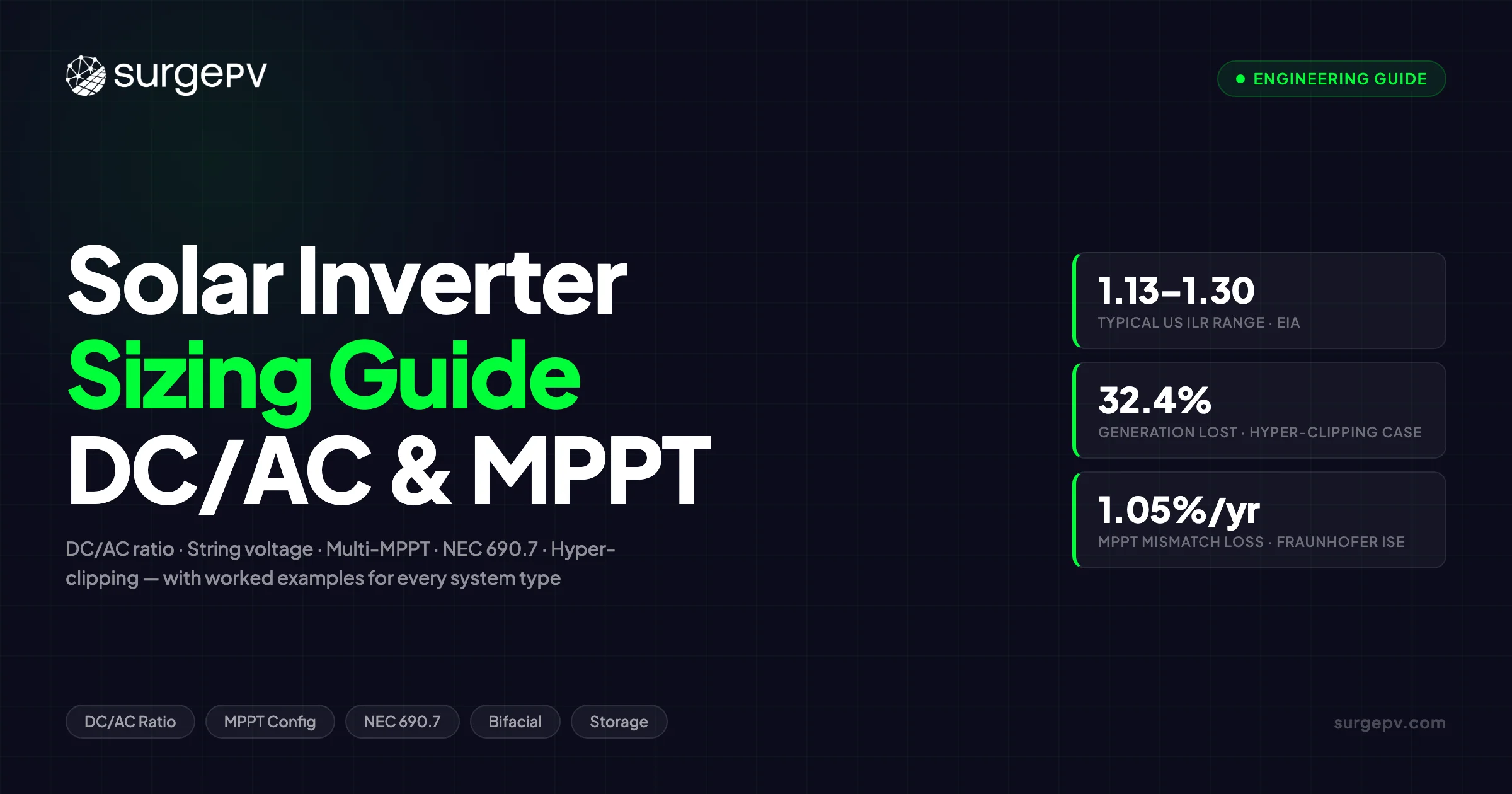
STC ratings assume 1,000 W/m², 25°C cell temperature, and AM 1.5 spectrum. An 8 kW inverter captures nearly all of that, only clipping when conditions approach STC. The EIA reports that inverter loading ratios for US individual systems are usually between 1.13 and 1.30 (EIA, 2018).
A single sizing error can cost a system far more than the inverter upgrade it was meant to avoid. A Los Angeles rooftop with a DC/AC ratio of 1.50 and a miscalculated minimum string length lost 32.4% of annual generation — not from moderate clipping, but because hot-weather string voltage dropped below the MPPT minimum, shutting the inverter down during peak afternoon hours. An AHJ plan submission that uses STC open-circuit voltage instead of the NEC 690.7 cold-temperature-adjusted figure gets rejected, costing weeks. These are not edge cases. They happen on real projects, and they are preventable.
STC ratings assume 1,000 W/m², 25°C cell temperature, and AM 1.5 spectrum. An 8 kW inverter captures nearly all of that, only clipping when conditions approach STC. The EIA reports that inverter loading ratios for US individual systems are usually between 1.13 and 1.30 (EIA, 2018).
This guide goes well beyond DC/AC ratio 101. It covers the seven sizing steps that catch every fundamental error: inverter voltage limits and NEC 690.7 compliance, MPPT voltage range at both temperature extremes, current limits including cloud-edge enhancement, clipping economics and when clipping crosses into hyper-clipping territory. It also covers the adjustments that standard guides skip: bifacial rear-side gain, single-axis tracker ILR correction, DC-coupled versus AC-coupled battery sizing, and multi-MPPT mismatch loss quantification. The EIA reports that most US systems operate at an inverter loading ratio between 1.13 and 1.30 — this guide explains why, and how to find the right number for any specific project. Solar software automates all seven steps in seconds; manual calculation remains essential for understanding what the software is checking and why.
TL;DR: Inverter Sizing Quick Reference
The EIA reports most US systems operate at a DC/AC ratio of 1.13 to 1.30 (EIA, 2018). For residential, target 1.15–1.25. Utility-scale: up to 1.34 (NREL ATB, 2024). String voltage must stay below NEC 690.7 limits — 600 V residential, 1,000 V commercial. Software simulates all of this in seconds; manual math catches the fundamentals but misses hourly clipping dynamics.
What this guide covers:
- How to choose the right DC/AC ratio for residential, C&I, utility, and SAT systems — with NREL and EIA benchmarks
- Cold-temperature Voc and hot-temperature Vmp string length calculations, step by step
- How to configure multi-MPPT inputs for mixed orientations and minimize mismatch losses
- Why bifacial modules change the optimal ILR — and by how much
- NEC 690.7 voltage limits for residential, commercial, and utility-scale systems
- Hybrid and battery inverter sizing: DC-coupled vs AC-coupled and the 1.5–1.8 ILR case
- When clipping becomes hyper-clipping — and a real LA project that lost 32.4% annually
- How design software automates string sizing, clipping simulation, and MPPT assignment
Step 1: Understand the DC-to-AC Ratio
The DC/AC ratio — also called the inverter loading ratio (ILR) — is the ratio of total DC array capacity to the inverter’s AC output rating.
DC/AC Ratio = Total DC Panel Capacity (Wp) ÷ Inverter AC Rating (W)
A 10 kWp array connected to an 8 kW inverter has a DC/AC ratio of 1.25.
Why Oversize the Array?
Solar panels almost never produce full rated power in the field. STC ratings assume 1,000 W/m², 25°C cell temperature, and AM 1.5 spectrum. Real conditions are different:
- Irradiance averages 700–850 W/m² over the daily production window on most sites
- Cell temperatures run 55–70°C, reducing output by 10–20% relative to STC
- Soiling, wiring losses, and mismatch reduce DC output by another 2–5%
A 10 kWp array typically delivers 7.5–8.5 kW DC under these conditions. An 8 kW inverter captures nearly all of that, only clipping when conditions approach STC. Adding DC panel capacity costs less per watt than adding inverter AC capacity. The cost savings on the DC side outweigh the small energy lost to clipping across the inverter’s lifetime.
Target DC/AC Ratios by Application
| Application | Typical DC/AC Ratio | Key Driver |
|---|---|---|
| Residential (non-MLPE) | 1.15 | NEC 600 V limit constrains string options |
| Residential (MLPE/optimizers) | 1.15–1.25 | Module-level electronics allow more flexibility |
| Commercial rooftop | 1.20–1.30 | Daytime load matching, higher capacity factor |
| Utility ground-mount (fixed-tilt) | 1.25–1.34 | Maximize capacity factor; NREL ATB 2024 default = 1.34 |
| Utility SAT (single-axis tracker) | 1.30 | Extended morning/evening harvest; NREL benchmark |
| High-irradiance (desert, tropical) | 1.10–1.20 | Frequent near-STC irradiance; more clipping risk |
| Low-irradiance (northern Europe) | 1.25–1.35 | Rare peak irradiance; minimal clipping |
| Hybrid (DC-coupled battery) | 1.40–1.80 | Battery absorbs clipped DC power |
Pro Tip
A RatedPower study of a 50 MWac plant in Germany found the optimal DC/AC ratio for the lowest LCOE was 1.18 (~49.3 €/MWh). Going higher added clipping losses faster than it reduced inverter cost. The optimal ratio is always site-specific — irradiance profile, land cost, and inverter pricing all shift the breakeven point.
Read more about Community Solar Projects Germany.
Three common mistakes when selecting a DC/AC ratio:
- Setting ILR = 1.0 to “avoid clipping” — this results in an oversized, more expensive inverter that runs well below its rated output for most of the year
- Applying the same ILR to a desert site and a Scottish site without adjusting for the irradiance profile — the optimal ratio differs by 0.10–0.20 between these climates
- Ignoring MLPE when setting ILR — module-level power electronics change the string voltage rules and allow ratios that would otherwise violate NEC 600 V limits
Step 2: Check Inverter Maximum DC Voltage
This is the most safety-critical step. If the string’s open-circuit voltage exceeds the inverter’s maximum DC input voltage, the inverter will not start and may be permanently damaged.
Why Cold Temperature Matters
Solar panel voltage increases as temperature drops. The worst case is a cold, clear winter morning when cells generate full Voc near ambient temperature. This is also the exact calculation that NEC 690.7 requires — the full compliance treatment is in the code compliance section below.
The Formula
Voc_max = Voc_STC × [1 + (T_min − 25) × (TK_Voc ÷ 100)]
Where:
- Voc_STC = open-circuit voltage at standard test conditions (from the panel datasheet)
- T_min = lowest expected ambient temperature at the site (°C)
- TK_Voc = temperature coefficient of Voc (negative %/°C, from the datasheet)
- 25 = STC reference temperature
Worked Example: Jinko Tiger Neo JKM420N-54HL4 at -10°C
Panel specifications (from Jinko Solar datasheet):
- Voc at STC: 38.54 V
- TK_Voc: -0.25%/°C
- Corrected Isc at STC: 13.59 A (datasheet-matched, JKM420N-54HL4 base variant)
Site minimum temperature: -10°C
Voc_max = 38.54 × [1 + (-10 − 25) × (-0.25 ÷ 100)] Voc_max = 38.54 × [1 + (-35) × (-0.0025)] Voc_max = 38.54 × [1 + 0.0875] Voc_max = 38.54 × 1.0875 Voc_max = 41.91 V per panel
Second example at -20°C for Scandinavia: Voc_max = 38.54 × [1 + (-20 − 25) × (-0.0025)] = 38.54 × 1.1125 = 42.87 V per panel
Maximum Panels Per String
Max panels = Inverter max DC voltage ÷ Voc_max (round DOWN)
| Inverter | Max DC Voltage | Max Panels at -10°C (41.91 V) | Max Panels at -20°C (42.87 V) |
|---|---|---|---|
| Fronius Symo GEN24 10.0 | 1,000 V | 1,000 ÷ 41.91 = 23 panels | 1,000 ÷ 42.87 = 23 panels |
| Huawei SUN2000-10KTL-M1 | 1,100 V | 1,100 ÷ 41.91 = 26 panels | 1,100 ÷ 42.87 = 25 panels |
| SolarEdge SE10K (with S440 optimizers) | 750 V (string) | Optimizer-regulated; use SolarEdge design tool | Optimizer-regulated |
SolarEdge Exception
SolarEdge systems with S440 power optimizers regulate each panel’s output voltage independently. The string voltage is determined by the number of optimizers, not panel Voc. The cold-temperature Voc calculation above does not apply directly. Use the SolarEdge design tool for string length limits — typically a maximum of 6,000 W per string for residential optimizers.
Temperature by Region
| Region | Recommended T_min | Source |
|---|---|---|
| Mediterranean | -5 to 0°C | ASHRAE 99.6% |
| Central Europe | -10 to -15°C | DWD / ASHRAE |
| Scandinavia | -20 to -30°C | SMHI / ASHRAE |
| US Southeast | -5 to -10°C | NOAA |
| US Mountain West | -15 to -25°C | NOAA |
| India / Gulf | 0 to +5°C | IMD |
Use the lowest recorded temperature for the site, not the average winter minimum. Sources: national meteorological data, TMY files, or ASHRAE 99.6% design temperatures.
What Happens When Voltage Is Exceeded
If string Voc exceeds the inverter’s maximum DC input voltage, the IGBT or MOSFET input stage can fail permanently. This is not a soft performance boundary — it is a hard equipment failure. AHJ plan reviewers verify this calculation. A submission that uses STC Voc instead of T_min-adjusted Voc is rejected.
Common mistake: using the average winter minimum instead of the design-day minimum. For a Hamburg site, the difference between the average winter low (-5°C) and the ASHRAE 99.6% design temperature (-15°C) shifts Voc_max by 1.5 V per panel — enough to change the maximum string length by one panel.
Step 3: Check MPPT Voltage Range
The inverter’s MPPT operates within a specific voltage window. If string voltage drops below the minimum, the inverter reduces output or shuts down entirely.
Cell Temperature vs. Ambient — NOCT Model
Solar panel voltage decreases as temperature rises. Worst case: a hot summer afternoon with a flush-mounted rooftop array.
Standard approximation (conservative):
- T_cell = T_ambient + 25 to 30°C (well-ventilated roof mounts)
- T_cell = T_ambient + 35 to 40°C (flush-mounted or poorly ventilated)
NOCT-based model (more accurate): T_cell = T_ambient + (NOCT − 20) ÷ 800 × G
Where G = plane-of-array irradiance in W/m² and NOCT is the Nominal Operating Cell Temperature from the panel datasheet (typically 43–46°C for modern panels).
Example: 35°C ambient, G = 800 W/m², NOCT = 43°C → T_cell = 35 + (43 − 20) ÷ 800 × 800 = 35 + 23 = 58°C. The NOCT model gives 58°C; the rule-of-thumb gives 70°C. The rule-of-thumb is conservative — which is fine for string sizing, where the conservative direction (lower Vmp) sets the minimum string length.
The Formula
Vmp_min = Vmp_STC × [1 + (T_cell_max − 25) × (TK_Vmp ÷ 100)]
If the datasheet lists TK_Vmp, use it. If only TK_Voc is listed, use it as a conservative proxy — both are negative and close in magnitude for crystalline silicon.
Worked Example: Jinko Tiger Neo JKM420N-54HL4 at 65°C Cell Temperature
Panel specifications:
- Vmp at STC: 31.97 V
- TK_Voc: -0.25%/°C (used as proxy for TK_Vmp)
Vmp_min = 31.97 × [1 + (65 − 25) × (-0.0025)] Vmp_min = 31.97 × [1 + 40 × (-0.0025)] Vmp_min = 31.97 × [1 − 0.10] Vmp_min = 31.97 × 0.90 Vmp_min = 28.77 V per panel
Minimum Panels Per String
Min panels = Inverter MPPT minimum voltage ÷ Vmp_min (round UP)
| Inverter | MPPT Min Voltage | Min Panels (Jinko 420W at 65°C cell temp) |
|---|---|---|
| Fronius Symo GEN24 10.0 | 80 V (MPPT operating minimum) | 80 ÷ 28.77 = 2.78 → 3 panels |
| Huawei SUN2000-10KTL-M1 | 200 V | 200 ÷ 28.77 = 6.95 → 7 panels |
| SMA Sunny Tripower 10.0 | 150 V | 150 ÷ 28.77 = 5.21 → 6 panels |
| Sungrow SG10RT | 200 V | 200 ÷ 28.77 = 6.95 → 7 panels |
| SolarEdge SE10K | Optimizer-based | Use SolarEdge design tool |
Fronius MPPT Voltage Note
Fronius GEN24 datasheets list a 65 V start-up voltage and an 80 V MPPT operating minimum. Use 80 V for string sizing — the inverter will not track MPPT below this point even if it starts up. Using 65 V understates the minimum string length by one panel in some configurations.
MPPT Tracking Accuracy Near Voltage Limits
Most inverters achieve peak MPPT efficiency in the middle 60–80% of their voltage window. Operating within 10% of either limit reduces tracking efficiency by 0.5–1.0%. Leave at least 10% headroom above the MPPT minimum at maximum cell temperature as a design margin.
Step 4: Determine Optimal String Length
With maximum and minimum string lengths established, the optimal length targets the center of the MPPT voltage window.
The Sweet Spot
Target: string Vmp at STC falls in the 60–80% range of the MPPT voltage window
Operating outside this range costs 0.5–1.0% in MPPT tracking efficiency per 10% deviation from center. For most systems, this is a minor loss — but it stacks with other system losses.
Worked Examples: Three Popular Inverter Combinations
Using Jinko Tiger Neo JKM420N-54HL4 panels with three common inverter options:
Combination 1: Fronius Symo GEN24 10.0 Plus
- MPPT operating range: 80 to 800 V; max DC input: 1,000 V
- Max panels per string (at -10°C): 23; Min panels (at 65°C): 3
- Target Vmp range (60–80% of window): 208 to 640 V
- Practical optimal: 9 to 17 panels
Combination 2: Huawei SUN2000-10KTL-M1
- MPPT range: 200 to 800 V (full power); max DC: 1,100 V
- Max panels (at -10°C): 26; Min panels (at 65°C): 7
- Target Vmp range: 350 to 600 V
- Practical optimal: 13 to 19 panels
Combination 3: SolarEdge SE10K with S440 Optimizers
- Max 6,000 W per string: 6,000 ÷ 420 = 14 panels max; min ~8 per SolarEdge guidelines
- Optimizer-based voltage regulation replaces the Voc/Vmp calculation
| Inverter | Min Panels | Max Panels | Practical Optimal |
|---|---|---|---|
| Fronius Symo GEN24 10.0 | 3 | 23 | 9 to 17 |
| Huawei SUN2000-10KTL-M1 | 7 | 26 | 13 to 19 |
| SolarEdge SE10K + S440 | 8 | 14 | 8 to 14 |
Unequal String Lengths: When to Use Dual MPPT
If two strings differ by more than 1–2 panels and share a single MPPT input, the tracker settles at a compromise operating point. The annual yield cost is 1–3%. Most modern inverters have 2 or 3 MPPT inputs to handle this.
Common inverters with dual MPPT: Fronius GEN24 (2 MPPT), Huawei SUN2000-M1 (2 MPPT), SMA STP 10.0 (2 MPPT), Sungrow SG10RT (2 MPPT).
For wiring configuration and series/parallel rules, see the solar panel stringing and wiring guide. For the broader residential design workflow, see how to design a residential solar system.
Pro Tip
When you have a 12-panel string and a 10-panel string that must coexist on the same inverter, put them on separate MPPT inputs rather than trying to match them. The 2-panel difference shifts Vmp by ~64 V — large enough that a single shared MPPT costs measurable yield.
Step 5: Check Current Limits
Each MPPT input has a maximum current rating. Exceeding it does not always damage the inverter, but it forces the MPPT to operate away from the optimal power point and can accelerate thermal aging on the input stage.
Single String Current
The relevant value is Isc at STC — not Imp. Isc is the value that determines the worst-case current the string can deliver, including under irradiance spikes above 1,000 W/m².
For Jinko Tiger Neo JKM420N-54HL4: Isc at STC = 13.59 A (datasheet-corrected value).
Cloud-Edge Enhancement: The Hidden Current Risk
Cloud-Edge Enhancement
When a cloud edge passes over a solar array, circumsolar radiation combines with direct irradiance to spike plane-of-array irradiance above the 1,000 W/m² STC reference. Field measurements show peaks of 29% above STC Prated — up to 1,290 W/m². Sandia National Laboratories data show approximately 7% of enhancement events last longer than 1 minute. At 1,290 W/m², the Jinko panel’s Isc scales to 13.59 × 1.29 ≈ 17.5 A.
This is why NEC 690 and inverter manufacturers require sizing to 1.25 × Isc_STC rather than Isc_STC alone. The 1.25 safety factor is partly a cloud-edge allowance.
Two parallel strings near the per-MPPT current limit illustrates the risk:
- Two strings in parallel: 13.59 × 2 = 27.18 A at STC
- Right at the limit for a Huawei SUN2000-10KTL-M1 input at its rated 13.5 A per MPPT for two parallel strings
- During a cloud-edge event: 17.5 × 2 = 35.0 A — 29% over the limit
Best practice: 1.25 × total Isc_STC must stay below the per-MPPT current rating.
Parallel Strings on One MPPT
| Inverter / MPPT Input | Max Input Current | Max Parallel Strings (Jinko JKM420N, Isc = 13.59 A) |
|---|---|---|
| Fronius GEN24 10.0 per MPPT | 25 A | 1 string (25 A ÷ 13.59 A = 1.84; floor = 1) |
| Huawei SUN2000-10KTL-M1 per MPPT | 13.5 A per string / 27 A total | 1 string with margin; 2 at STC only |
| Huawei SUN2000-50KTL-M3 per MPPT | 32 A | 2 strings |
| Commercial 3-phase (typical) | 40–50 A | 2–3 strings |
Temperature Effect on Isc
Isc increases approximately +0.05%/°C for mono-PERC and TOPCon panels — a small addition that stacks with cloud-edge enhancement at peak irradiance. Account for this when calculating current margins for hot-climate installations.
Step 6: Account for Inverter Clipping
Clipping occurs when DC power exceeds the inverter’s maximum AC output. The inverter shifts its operating point away from maximum power, reducing DC input to match the AC limit.
What Clipping Looks Like
On a clear summer day for a 10 kWp array / 8 kW inverter (DC/AC = 1.25):
| Time | DC Output | AC Output | Clipped |
|---|---|---|---|
| 8:00 AM | 4.0 kW | 4.0 kW | 0 kW |
| 10:00 AM | 7.5 kW | 7.5 kW | 0 kW |
| 12:00 PM | 9.8 kW | 8.0 kW | 1.8 kW |
| 2:00 PM | 9.2 kW | 8.0 kW | 1.2 kW |
| 4:00 PM | 6.5 kW | 6.5 kW | 0 kW |
The clipped energy is lost, but the inverter runs at or near full capacity for more hours than a 1.0 DC/AC system would, producing more total annual energy.
Acceptable vs. Excessive Clipping
| DC/AC Ratio | Typical Annual Clipping Loss | Assessment |
|---|---|---|
| 1.00–1.10 | 0% | No clipping — inverter is likely oversized |
| 1.10–1.20 | 0–1% | Minimal; common for high-irradiance sites |
| 1.20–1.30 | 1–2% | Optimal for most residential and commercial projects |
| 1.30–1.40 | 2–4% | Acceptable for utility-scale with cheap DC capacity |
| 1.40–1.50 | 4–7% | Aggressive; needs a detailed financial model |
| Above 1.50 | 7%+ | Excessive without DC-coupled battery storage |
These values assume a temperate climate (central Europe or mid-latitude US). High-irradiance sites see higher clipping at the same ratios; low-irradiance sites see lower clipping.
NREL SAM Clipping Methodology
SAM models two types of clipping: power clipping (inverter saturation at its nameplate AC rating) and MPPT clipping (input voltage outside the MPPT range). The Allen and Walker subhourly correction methods (NREL/CP-7A40-90237) produce annual energy estimates accurate to ±2% compared to 1-minute interval simulation.
Key finding from NREL: hourly simulation understates clipping in climates with frequent transient irradiance spikes. Sub-hourly simulation (5- or 15-minute intervals) is more accurate for desert sites with cloud-edge events. For residential and commercial in temperate climates, hourly SAM simulation is sufficient. For utility-scale in the US Southwest or Middle East, request sub-hourly clipping analysis.
PVsyst accepts 0.2–3% overload loss as normal. Losses above 3% trigger a financial review in most bankable energy assessments.
The Economics of Clipping
For a 10 kWp / 8 kW system (DC/AC = 1.25):
- Annual production without clipping: 11,000 kWh
- Clipping loss at 1.25 ratio: ~1.5% = 165 kWh
- Value of lost energy at €0.10/kWh: €16.50/year
- Cost of upgrading to a 10 kW inverter: €300–€500
- Simple payback on the upgrade: 18–30 years
The math does not support sizing the inverter larger just to eliminate clipping at this ratio.
Pro Tip
DC-coupled battery systems change the clipping economics entirely. Clipped DC power goes to the battery rather than being wasted. At a DC/AC ratio of 1.40–1.50 with DC-coupled storage, the “lost” energy is mostly recovered — see the Battery Inverter Sizing section below.
For more on this topic, see AC Coupled vs DC Coupled Battery Solar.
When Clipping Becomes a Problem
Clipping above 5% annually warrants closer analysis. Warning signs:
- Flat-topped production curves lasting more than 4 hours on clear days
- Revenue loss exceeding the cost of a reasonable inverter upgrade
- Grid curtailment stacking — see the Grid Export Limits section below
- Hyper-clipping risk — see the Hyper-Clipping Warning section below
Use the generation and financial tool to model clipping losses against your energy price, feed-in tariff, and self-consumption rate before finalizing the inverter size.
Step 7: Let Design Software Handle the Math
Manual string sizing works cleanly for single-orientation, unshaded systems. It gets complicated with multiple roof faces, seasonal temperature extremes, and bifacial panels.
What solar design software handles that manual calculation cannot:
Automatic string configuration. Given a panel and inverter model, the software calculates all valid string lengths, checks limits at both temperature extremes, and proposes optimal wiring — including which strings go on which MPPT input.
Hourly clipping simulation. The software models DC production for every hour against the inverter AC limit, capturing seasonal variation that lookup tables miss.
Multi-MPPT optimization. East- and west-facing strings go on separate MPPT inputs automatically. Mismatch loss is quantified before installation.
Bifacial rear-gain correction. Manual calculation ignores rear-side irradiance because it needs a 3D irradiance model. Software that incorporates rear-irradiance modeling adjusts the effective DC/AC ratio for bifacial panels.
SAT DC/AC adjustment. Single-axis tracker power curves need a different ILR than fixed-tilt. Software applies the -0.05 to -0.10 correction based on tracker geometry.
Temperature-adjusted yield modeling. Hourly TMY temperature data produces tighter results than manual worst-case temperatures alone.
For panel layout planning, see the solar panel layout design guide. For the full design-to-proposal workflow, solar proposal software integrates sizing outputs into client-ready proposals.
Auto-Size Inverters, Strings, and MPPT in Minutes
SurgePV checks voltage limits, current limits, MPPT mismatch, and clipping losses automatically for any panel and inverter combination — including bifacial rear-gain correction and SAT DC/AC adjustment.
Book a DemoNo commitment required · 20 minutes · Live project walkthrough
Results: Complete Sizing Walkthrough
Project: 8.4 kWp rooftop system in Hamburg, Germany (53.5°N, annual GHI ~950 kWh/m²) Also see: Germany solar subsidies.
Equipment: 20 × Jinko Tiger Neo JKM420N-54HL4 (420 Wp each, total 8,400 Wp)
Step 1 — DC/AC Ratio: Initial pick: Huawei SUN2000-8KTL-M1 (8.0 kW). DC/AC = 8,400 ÷ 8,000 = 1.05 — below optimal for Hamburg’s low-irradiance climate. A 7 kW inverter (SUN2000-7KTL-M1) gives DC/AC = 8,400 ÷ 7,000 = 1.20. That is the right match for Hamburg.
What goes wrong with the 8 kW inverter: The inverter runs at 75% of rated capacity on most production days. Inverter efficiency peaks at 95–100% of rated output; sustained partial-load operation increases thermal cycling and accelerates component aging. Annual yield is approximately 4% lower than the 7 kW option. The 8 kW inverter is larger and more expensive — and produces less energy.
Step 2 — Max string length (cold): T_min Hamburg: -15°C (ASHRAE 99.6% design temperature). Voc_max = 38.54 × [1 + (-15 − 25) × (-0.0025)] = 38.54 × 1.10 = 42.39 V/panel Max panels = 1,100 ÷ 42.39 = 25 panels. No constraint here — 20 panels total fit comfortably.
Step 3 — Min string length (hot): T_cell_max: 35°C ambient + 30°C (ventilated roof mount) = 65°C Vmp_min = 31.97 × [1 + (65 − 25) × (-0.0025)] = 31.97 × 0.90 = 28.77 V/panel Min panels = 200 ÷ 28.77 = 6.95 → 7 panels (round up)
Step 4 — String configuration: 20 panels total. Valid range: 7 to 25 per string. Two strings of 10 panels: Vmp_STC = 31.97 × 10 = 319.7 V — within the 200–800 V MPPT window. Good.
MPPT assignment: Even a mostly south-facing Hamburg rooftop typically has slight azimuth variation between the two slopes. Each string of 10 panels gets its own MPPT input. The SUN2000-7KTL-M1 has 2 MPPT inputs — the right choice. Each tracker independently finds its peak during partly cloudy conditions. Assigning both strings to a single MPPT would cost up to 1.0%/year per Fraunhofer ISE field data.
Step 5 — Current check: Isc = 13.59 A per string. Huawei SUN2000-7KTL max input per MPPT: 13.5 A per string. One string per MPPT: 13.59 A — within spec. Cloud-edge check: 1.25 × 13.59 = 16.99 A — below the single-string 13.5 A per-MPPT limit? Actually 13.59 A is close to the 13.5 A per-string limit — note this to the client. The inverter’s overcurrent protection will engage during cloud-edge events on this specific combination.
Step 6 — Clipping estimate: DC/AC = 1.20 in Hamburg (annual GHI ~950 kWh/m²). Expected annual clipping: under 0.5%. Negligible.
Final configuration: 2 strings of 10 panels, each on a separate MPPT input. Inverter: Huawei SUN2000-7KTL-M1. DC/AC = 1.20. Annual clipping under 0.5%.
MPPT Multi-Tracker Configuration: Orienting Strings by Azimuth and Tilt
What Is MPPT Mismatch Loss?
When two strings with different irradiance profiles — different azimuth, tilt, or shading — share one MPPT input, the tracker finds a single operating point that works for neither string at its peak. That is MPPT mismatch loss.
Fraunhofer ISE (2021) measured worst-case mismatch loss for a poorly assigned single-MPPT system at 1.05% per year. Correct multi-MPPT assignment — each distinct orientation on its own tracker — drops mismatch loss to 0.3–1.0%/year. For an 8 kWp system producing 8,000 kWh/year, the 1.05% difference is 84 kWh annually. At €0.10/kWh that is €8.40/year — small, but avoidable with a configuration change that costs nothing.
The Rule: One Orientation Per MPPT
- East-facing strings → MPPT 1
- West-facing strings → MPPT 2
- South-facing strings → either MPPT, or a third input if available
- Dual-pitch roofs with different tilts (e.g., 30° and 15°): assign separately when the inverter has the inputs available
For three-orientation systems, put the pair with the most similar irradiance profile on the same MPPT. East + West on one MPPT is worse than South + East, because east and west peak at opposite ends of the day.
See the solar angles and azimuth guide for azimuth and tilt reference data by location.
Worked Example: East-West Split Roof
System: 10 panels east (azimuth 90°, tilt 20°), 10 panels west (azimuth 270°, tilt 20°). Total 8.4 kWp.
If both strings share one MPPT: the tracker runs at the mean operating voltage of two strings that peak at opposite times of day. Yield from both strings drops 2–4% annually.
If each string gets its own MPPT: the east tracker finds its peak in the morning; the west tracker finds its peak in the afternoon. Full harvest from both.
Current Limits Still Apply Per MPPT
Correct MPPT assignment does not waive the current check from Step 5. Verify Isc per string against the per-MPPT input limit for each individual input.
Common Mistake
Running an east string and a north string on the same MPPT. The north string barely produces at midday while the east string is near peak. The MPPT compromise is severe. Assign the north string its own input — or consider whether a north-facing string is worth including at all.
Bifacial Module Inverter Sizing: Bifaciality Factor and Rear-Side Gain
Bifacial Gain Basics
Bifacial modules generate electricity from both front and rear sides. The bifaciality factor — the ratio of rear-to-front efficiency — ranges from 0.65 to 0.80 for most current commercial modules. NREL ATB 2024 projects this reaching 0.85 by 2035 for advanced scenarios.
Field-measured rear-side gain: typically 5–15% above front-only nameplate power, depending on mounting height, row spacing, and ground albedo. A 420 Wp front-side module with 70% bifaciality factor and 10% rear gain produces approximately 462 Wp under representative conditions — even though the datasheet shows 420 Wp.
Why the Optimal ILR Is Lower for Bifacial Systems
Most designers size the inverter to the nameplate DC capacity. With bifacial panels, the effective DC/AC ratio is higher than that nameplate implies — the array produces more power than the datasheet suggests, pushing real-world clipping losses above the modeled forecast.
NREL guidance: “The optimal ILR of PV systems in higher resource classes or for those that use bifacial modules will be lower than the optimal ILR of systems with monofacial modules, particularly without the use of energy storage.”
The correction: reduce the target ILR by 0.05–0.10 from the monofacial baseline.
Scenario Comparison
| Module Type | Nameplate Wp | Effective Wp (with rear gain) | Recommended ILR | Annual Clipping (central EU) |
|---|---|---|---|---|
| Monofacial 420W | 420 | 420 | 1.25 | ~1.5% |
| Bifacial 420W (10% rear gain) | 420 | 462 | 1.16 | ~1.5% |
| Bifacial 420W (15% rear gain) | 420 | 483 | 1.11 | ~1.5% |
To maintain equivalent clipping at the same inverter size, recalculate ILR using the bifacial-corrected effective Wp.
Practical Guidance
Default rear-gain estimates by surface type:
- Elevated ground-mount with concrete or gravel (15–25% albedo): 5–8% rear gain
- Snow-prone ground or white membrane rooftop (30–50% albedo): 10–12% rear gain
- Flush rooftop mount: ~0% rear gain (rear face blocked by roofing material)
Request rear-irradiance modeling from solar design software when specifying bifacial panels — manual calculation ignores rear-side geometry entirely.
Warning: applying a standard 1.25 ILR to a bifacial ground-mount system without rear-gain correction is one of the most common oversizing errors in utility-scale project finance models.
Single-Axis Tracker DC/AC Ratio
Why SAT Systems Use a Lower ILR Than Fixed-Tilt
Single-axis trackers rotate the panel plane to follow the sun across the day. The result: a flatter, wider daily power curve. The peak is lower than a fixed-tilt south-facing array at solar noon — panels never simultaneously reach the optimal angle. But energy delivery extends further into morning and afternoon.
NREL ATB 2024 benchmark: SAT ILR = 1.30 vs fixed-tilt utility-scale = 1.34. Industry practice (PV-Maps, GreenTechRenewables): apply -0.05 to -0.10 to the fixed-tilt baseline when specifying SAT.
Because SAT panels never simultaneously hit peak irradiance at solar noon, the power curve peak is lower. There is less benefit to aggressive DC oversizing because the inverter runs near rated output through more hours without needing a high ILR.
The SAT Clipping Profile
SAT systems clip less at solar noon but more during shoulder hours when the tracker maximizes harvest. This extended production benefits from a slightly lower ILR.
Numeric comparison: for a 10 MWac SAT plant, ILR 1.30 vs 1.34 produces approximately 0.8–1.2% more annual energy at the lower ratio due to reduced shoulder-hour clipping. At 100 MWac, this difference is 0.8–1.2 GWh/year. For France-specific information, see Agricultural Solar Case Study.
Interaction with Backtracking
Modern SAT controllers use backtracking to reduce row-to-row shading at low sun angles. Backtracking briefly reduces irradiance on the panel face during morning and evening. This slightly supports a marginally higher ILR (closer to 1.34 rather than 1.30). The effect is site-specific — request energy simulation with actual tracker control parameters, not generic SAT assumptions.
SAT + Bifacial: The Most Common Utility Configuration
Target ILR: approximately 1.20–1.25.
- SAT baseline: 1.30
- SAT correction vs. fixed-tilt: -0.05
- Bifacial correction: -0.05 to -0.09 (depending on rear gain)
Applying fixed-tilt monofacial ILR (1.34) to a SAT bifacial system without correction results in 3–5% more annual clipping than modeled at financial close.
Hybrid and Battery Inverter Sizing: DC-Coupled vs AC-Coupled Storage
DC-Coupled Storage: Higher ILR Is Justified
In a DC-coupled system, the battery charge controller sits on the DC bus between the array and the inverter. Clipped DC power — energy that would otherwise be wasted when array DC exceeds the inverter’s AC limit — goes to the battery instead.
Round-trip efficiency for DC-coupled storage: 95–98% (single conversion path).
With DC-coupled storage, an ILR of 1.40–1.50 for residential and 1.50–1.80 for large C&I is financially justified. The clipped energy is stored and dispatched in the evening. DC-coupled clipping recapture can boost annual system yield by 8–12% relative to a system without storage at the same ILR.
AC-Coupled Storage: ILR Rules Unchanged
In an AC-coupled system, the battery inverter sits on the AC bus. The main inverter still clips at its rated AC output. Clipped energy cannot be captured — the main inverter is the binding constraint regardless of battery size.
AC-coupled round-trip efficiency: 85–92% (two conversion steps).
For AC-coupled systems, apply the same ILR guidance as a system without storage.
DC-Coupled ILR Sizing Comparison
| System | Array DC | Inverter AC | Battery | ILR | Est. Annual Benefit |
|---|---|---|---|---|---|
| Residential (AC-coupled) | 10 kWp | 8 kW | 10 kWh | 1.25 | Clipping is lost |
| Residential (DC-coupled) | 12 kWp | 8 kW | 10 kWh | 1.50 | 8–12% yield boost |
| C&I (DC-coupled) | 200 kWp | 130 kW | 150 kWh | 1.54 | Up to 12% yield boost |
Hybrid Inverter Sizing Specifics
All-in-one hybrid inverters (Sungrow SH series, Huawei SUN2000 with LUNA2000) have separate PV input and battery port ratings.
Size the PV input ILR against the inverter’s PV input rating — not the total system output rating. Verify the battery port’s maximum charge rate: some residential hybrid inverters cap battery charging at 5 kW even when the PV array is 12 kWp. If the ILR exceeds 1.50, confirm the battery port can absorb peak clipping power — otherwise excess DC is still wasted.
NEC 690.7 and IEC 62109 Compliance: Voltage Limits by System Type
NEC 690.7 Maximum DC Voltage
NEC 690.7 sets maximum system voltage for PV arrays connected to buildings:
| System Type | NEC 690.7 Max DC Voltage |
|---|---|
| Residential (one- and two-family dwellings) | 600 V |
| Commercial / multi-family / non-dwelling | 1,000 V |
| Utility ground-mount (non-dwelling) | 1,500 V |
NEC 690.7 requires string Voc to be calculated at the record low temperature for the site using the Voc temperature coefficient from the panel datasheet — exactly the calculation in Step 2. The 600 V residential limit explains why US residential string inverters top out at 600 V DC input while European residential inverters reach 1,000 V.
Compliance and Plan Check
AHJ plan reviewers verify the cold-temperature Voc calculation. Submissions using STC Voc instead of T_min-adjusted Voc are rejected.
Common rejection scenario: 16 panels × Voc_STC 37.5 V = 600 V. Looks compliant at first glance. At -10°C: Voc_cold = 40.78 V → string Voc = 652 V — exceeds the 600 V residential limit. Plan rejected. Fix: reduce to 14 panels (14 × 40.78 = 571 V) or switch to a commercial-class inverter rated for 1,000 V.
IEC 62109 — International Context
IEC 62109-1 and 62109-2 govern inverter safety in Europe, Australia, and most non-NEC markets. Maximum DC voltage: 1,000 V for grid-tied residential. Australia’s AS/NZS 5033 references 1,000 V for most systems, with 1,500 V permitted under additional requirements. For Australia-specific compliance details, see Australia comparisons/lgc-vs-stc.
The cold-temperature Voc calculation in Step 2 applies identically across NEC and IEC markets — only the voltage ceiling differs.
When 1,500 V Systems Apply (US)
Utility ground-mount projects increasingly use 1,500 V inverters and string combiners. At 1,500 V, string lengths can reach 30–35 panels for large-format modules.
Key compliance gap: all BOS components — wire insulation, string combiners, DC disconnects, fuses — must be rated for 1,500 V DC. This is where compliance failures most often appear in early-stage designs: 1,000 V-rated combiners substituted for 1,500 V components to cut cost.
Design Compliance Checklist
- Calculate Voc at the ASHRAE 99.6% heating design temperature for the project location
- Confirm string Voc stays below the applicable NEC 690.7 ceiling
- Confirm all BOS components match the system voltage class
- Document the temperature source (weather station ID or TMY file citation)
- Submit the cold-temperature Voc calculation worksheet with the permit set
Grid Export Limits and Curtailment Interaction
What Is Export Limiting?
Many grid operators cap the AC power a solar system can export. Germany’s EEG limits residential systems to 70% of peak power export. Australia’s DNSP rules vary by state. The UK’s G99 and G100 standards set limits for larger systems. For the latest details on UK, see Battery Solar System Design UK.
A 10 kWp system in Germany at 70% export = maximum 7 kW AC export.
Double Penalty: Clipping Plus Curtailment
If the inverter is sized to 8 kW AC (ILR = 1.25) and the grid export cap is 7 kW, two independent losses stack:
- Inverter clipping: any DC power above 8 kW AC equivalent is clipped
- Grid curtailment: any AC power above 7 kW is curtailed by the grid meter or inverter setting
Combined annual losses can reach 5–10%. This changes the ILR optimization. There is less reason to push ILR above 1.10–1.15 when export is already heavily curtailed, because added DC capacity increases losses in two places simultaneously.
Self-Consumption Offsets the Analysis
If the site has high daytime self-consumption — manufacturing, always-on HVAC, retail — export limiting matters less. Most generation is consumed before reaching the export cap.
For behind-the-meter C&I loads exceeding 70% of peak array power, ILR 1.25–1.30 remains optimal even with strict export limits.
Curtailment + Clipping Scenarios
| ILR | Export Cap | Inverter Clipping | Grid Curtailment | Combined Loss |
|---|---|---|---|---|
| 1.25 | None | ~1.5% | 0% | 1.5% |
| 1.25 | 70% Germany | ~1.5% | ~5% | ~6.5% |
| 1.10 | 70% Germany | ~0.5% | ~5% | ~5.5% |
| 1.10 | 70% + high self-consumption | ~0.5% | ~1% | ~1.5% |
The generation and financial tool models curtailment scenarios and optimizes ILR against effective revenue capture — not just total generation.
Partial Shading and MPPT Behavior: String Inverter vs Microinverter vs Optimizer
Why Shading Breaks String MPPT
A string inverter’s MPPT tracks one voltage point for the entire string. When one panel is shaded, it becomes the limiting element. Bypass diodes prevent a complete shutdown, but the shaded cell group is bypassed and string Vmp drops by approximately 10–12 V per bypassed group.
Partial shading creates multiple local maximum power points on the P-V curve. A single MPPT tracker may lock on the wrong local maximum, producing 10–25% less energy than an unshaded string.
Modern inverters with shade-tolerant global MPPT (Fronius, Huawei, Sungrow) periodically sweep the full voltage range to find the global maximum. This reduces shade-related mismatch to approximately 5–10% for moderate shading — but cannot eliminate it. For Global-specific compliance details, see Global net-metering-by-country.
Microinverters and Optimizers: MPPT Per Panel
Microinverters (Enphase IQ8 series) and DC optimizers (SolarEdge, Tigo) place an independent MPPT at each panel. A shaded panel operates at its own reduced maximum without affecting adjacent panels.
Yield advantage in partial shade: 10–25% more energy vs an unmitigated string inverter. See solar shadow analysis software for site shade assessment before specifying inverter technology.
Inverter Technology by Shading Level
| Shading Severity | Recommended Technology | Typical ILR Target |
|---|---|---|
| None or minimal (open field) | String inverter | 1.25–1.34 |
| Mild (one obstruction, brief) | String inverter with global MPPT | 1.20–1.25 |
| Moderate (tree, chimney, 1–3 hours/day) | DC optimizers | 1.20–1.25 |
| Severe (multi-source, 4+ hours/day) | Microinverters | 1.15–1.20 |
ILR Implications of MLPE
With per-panel optimization, the effective DC/AC ratio is more predictable. Shading no longer unpredictably shifts the string’s Vmp. The ILR calculation in Steps 1–5 stays valid; the shade-loss factor simply drops from ~15% (string inverter) to ~2% (MLPE).
Cloud-Edge Enhancement and Over-Irradiance
What Cloud-Edge Enhancement Is
When a cloud edge passes over a solar array, circumsolar radiation — light scattered around the cloud perimeter — combines with direct normal irradiance to briefly push plane-of-array irradiance above the 1,000 W/m² STC reference.
Field measurements: peaks of 29% above STC Prated — up to 1,290 W/m² — recorded on residential rooftop arrays. Sandia National Laboratories data show approximately 7% of enhancement events last longer than 1 minute. Most spikes last seconds.
Current and Voltage Implications
Isc scales approximately linearly with irradiance. At 1,290 W/m²:
- Jinko Tiger Neo JKM420N-54HL4 at cloud-edge: 13.59 × 1.29 ≈ 17.5 A
Voc changes negligibly with irradiance (logarithmic relationship). Cloud-edge Voc ≈ Voc_STC for practical sizing purposes.
This is why NEC 690 and inverter manufacturers require sizing to 1.25 × Isc_STC. The 1.25 safety factor is partly a cloud-edge allowance.
Design Risk: Parallel Strings Near the Current Limit
A common error: two parallel strings at 13.59 A each → 27.18 A → close to the 27 A MPPT limit on some inverters.
During a cloud-edge event: 17.5 × 2 = 35.0 A → 29% over the limit.
The inverter’s protection circuit engages. Repeated over-current events accelerate thermal aging on input capacitors. Best practice: 1.25 × total Isc_STC must stay below the per-MPPT current limit.
Climate Sensitivity
Cloud-edge events are most frequent in:
- Coastal and temperate continental climates: UK, Netherlands, US Great Lakes, New England, coastal California
- Tropical climates with afternoon convective clouds
Cloud-edge events are rare in desert climates (UAE, US Southwest, Atacama). In desert designs, the 1.25 × Isc margin is primarily a safety factor. In coastal Scotland, it is genuine real-world protection.
Designer Note
Cloud-edge enhancement is one reason a design review still adds value beyond software automation. Software may propose the theoretical maximum number of parallel strings; a site in coastal Scotland warrants an explicit current margin check before approval.
Hyper-Clipping Warning: When High DC/AC Ratios Collapse
What Hyper-Clipping Is
Hyper-clipping is not a high clipping percentage. It is a regime where the combination of high ILR, hot ambient temperatures, and a narrow MPPT voltage window causes string Vmp to fall below the MPPT minimum voltage — shutting the inverter down entirely during peak production hours.
At high temperatures, string Vmp decreases (Step 3). At high ILR, the inverter is saturated at its AC limit and cannot raise the operating voltage. When Vmp falls below the MPPT minimum, the inverter trips. Output goes to zero — not reduced, zero.
The loss is multiplicative: zero output × several hours = a large annual energy gap. Unlike normal clipping, which is continuous and predictable, hyper-clipping produces blocks of zero production on the hottest, highest-irradiance days.
The Los Angeles Case Study
Source: HelioScope / now.solar (2019), analysis of a real installed system. For software options, see 7 Best HelioScope Alternatives in.
- Array: 1.50 DC/AC ratio, south-facing rooftop in Los Angeles
- Problem: string Vmp at 65°C cell temperature dropped below the MPPT minimum for 4–6 hours on summer afternoons
- Annual result: 32.4% of potential generation lost — far beyond the 7–12% expected from normal clipping at a 1.50 ratio
The analysis found the effect multiplicative: high ILR and narrow MPPT window independently cause ~5.7% and ~0.6% losses. Combined: 32.4%. A Step 3 minimum string length check would have caught this before installation.
How to Detect Hyper-Clipping Risk Before Installing
Three checks:
- Vmp_hot check (Step 3): string Vmp at maximum cell temperature must stay at least 10% above the MPPT minimum voltage
- ILR stress check: model the hourly power curve on a typical hot summer day; if flat-top clipping exceeds 6 hours, the ILR is too aggressive for that climate
- Software validation: run hourly or sub-hourly simulation with TMY temperature data — solar software that models hourly cell temperatures gives a realistic clipping and MPPT behavior profile
The Risk Threshold
Hyper-clipping risk is material when all three conditions are true simultaneously:
- ILR above 1.40
- Maximum cell temperature above 70°C
- String Vmp_hot within 15% of the MPPT minimum voltage
Frequently Asked Questions
What is a good DC to AC ratio for solar?
For most residential systems, a DC/AC ratio of 1.15 to 1.25 delivers the best financial result. Commercial rooftop systems typically use 1.20 to 1.30, and utility-scale ground-mount systems can reach 1.34 (NREL ATB 2024). The right ratio depends on irradiance, module type, and whether battery storage is in play. Read Adding Battery Storage Services for a complete walkthrough.
How do you calculate solar inverter size?
Divide total DC array capacity in watts by the inverter AC rating to get the DC/AC ratio. Then verify: cold-temperature Voc stays below the inverter maximum DC input voltage (Step 2); hot-temperature Vmp stays above the MPPT minimum (Step 3); total string Isc stays below the per-MPPT current limit (Step 5). Run a clipping simulation to confirm annual losses below 3 percent.
What is inverter clipping and is it always bad?
Inverter clipping occurs when DC power from the array exceeds the inverter’s AC output capacity. At a DC/AC ratio of 1.25, annual clipping is typically 1 to 2 percent — below the breakeven point for a larger inverter. Clipping becomes a problem above 5 percent annually, or when combined with grid export curtailment.
What is the maximum DC voltage for residential solar?
In the US, NEC 690.7 limits residential PV systems to 600 V DC at the inverter input for one- and two-family dwellings. Commercial and industrial systems can reach 1,000 V. Utility ground-mount systems can reach 1,500 V when using listed 1,500 V-rated equipment. European markets under IEC 62109 allow 1,000 V for most residential and commercial systems.
How does battery storage change inverter sizing rules?
DC-coupled storage allows the array to run at a DC/AC ratio of 1.40 to 1.80 because clipped DC power charges the battery instead of being wasted, boosting annual yield by 8 to 12 percent. AC-coupled storage does not change inverter sizing rules — the main inverter is still the binding constraint.
What is MPPT mismatch loss and how do you minimize it?
MPPT mismatch loss occurs when strings with different irradiance profiles share a single MPPT input. Fraunhofer ISE (2021) measures worst-case mismatch at 1.05 percent per year. Correct multi-MPPT assignment — each distinct orientation on its own tracker — reduces this to 0.3 to 1.0 percent per year.
How do bifacial modules affect inverter sizing?
Bifacial panels produce 5 to 15 percent more energy than their nameplate watt-peak because of rear-side irradiance. To avoid more clipping than planned, reduce the target DC/AC ratio by 0.05 to 0.10 from the monofacial baseline. For fixed-tilt bifacial, use a DC/AC ratio of 1.20 to 1.28 instead of 1.25 to 1.30.
What is hyper-clipping and how do I avoid it?
Hyper-clipping occurs when a high DC/AC ratio combined with high summer temperatures causes string Vmp to fall below the inverter’s MPPT minimum voltage, shutting the inverter down during peak production hours. A Los Angeles project with a 1.50 DC/AC ratio and an incorrect string configuration lost 32.4 percent of annual generation. Verify minimum string length at maximum cell temperature (Step 3) before finalizing the design.
Manual sizing from these seven steps catches every fundamental error — cold Voc violations, MPPT range misses, current overloads, and clipping above the acceptable threshold. For a complete design with 3D layout, hourly clipping simulation, and a client-ready proposal, solar design platform handles the rest. Book a demo to see it on a real project.